
Evolution of Internet Congestion Control
The Physics behind your internet speed: A 40-Year Journey

On October 27, 1986, the ARPANET backbone experienced a four-hour outage that brought much of the early Internet to a standstill. The cause was not a hardware failure or a software bug, but a fundamental design flaw: TCP senders, lacking any sense of network capacity, would retransmit dropped packets aggressively, creating a feedback loop where dropped packets caused more retransmissions, which overwhelmed router buffers further, causing more drops. This was congestion collapse–a stable state where the network is fully utilized but delivers zero useful throughput.
This incident forced the realization that TCP needed a control mechanism. Not just reliability, but a way to sense how much data the network could carry and adjust sending rate accordingly. The subsequent forty years of development show a clear pattern: each major algorithm responded to the limitations of its predecessor by improving the quality of the signal used to estimate network state. The story is not one of revolutionary breakthroughs, but of incremental refinement driven by improvement in hardware capability and a deepening understanding of what can and cannot be measured in a distributed system.
Congestion Window
TCP does not directly control transmission rate. It controls congestion window size, or cwnd—the maximum amount of data that can be in flight, sent but not yet acknowledged. The actual sending rate is cwnd/RTT, where RTT is the round-trip time or the time taken by a packet to reach the destination and its acknowledgement packet to return back to the source host. To send faster, you increase cwnd. To send slower, you decrease it.
Every network path has a physical capacity called the Bandwidth-Delay Product (BDP). If the bottleneck bandwidth is 100 Mbps and the propagation delay (light speed plus fixed processing) is 50 ms, then:
BDP = 100 Mbps × 0.05 s = 5 Mb = 625 KB
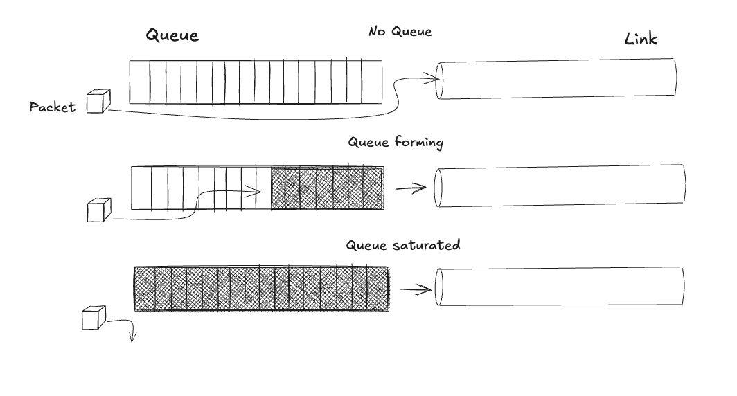
This value represents the ideal amount of data to keep in flight: enough to keep the bottleneck link fully busy, but not enough to create a queue. Any packet beyond the BDP sits in a buffer, adding delay without increasing throughput. A queued packet is wasted capacity.
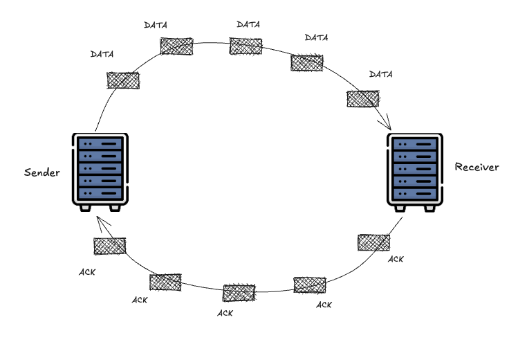
The ACK is your sensor. Each acknowledgment tells you that a packet has left the network, freeing one slot in your window. The arrival rate of ACKs is the network’s delivery rate. The time between sending a packet and receiving its ACK is the RTT, which includes propagation delay plus any queueing delay. The entire challenge of congestion control is to infer the path’s BDP from this single, noisy sensor.
TCP Tahoe:
In 1988, Van Jacobson implemented the first congestion control algorithm in BSD Unix. Given the hardware constraints—10 MHz CPUs, limited memory, no floating-point support—the logic was deliberately simple:
Slow Start: Begin with
cwnd = 1 MSS(Maximum Segment Size, typically 1460 bytes). For each ACK, increasecwndby 1 MSS. This doubles the window every RTT to find the rough capacity quickly.Congestion Avoidance: Once
cwndexceeds a threshold (ssthresh), switch to linear growth:cwnd += 1 MSS/cwnd, which adds roughly one MSS per RTT.Loss Reaction: On any loss (timeout or three duplicate ACKs), set
ssthresh = cwnd/2and resetcwnd = 1 MSS. Then re-enter slow start.
Why reset to 1? After congestion, the safe approach is to assume the network state is completely unknown. Resetting guarantees you cannot cause another collapse.
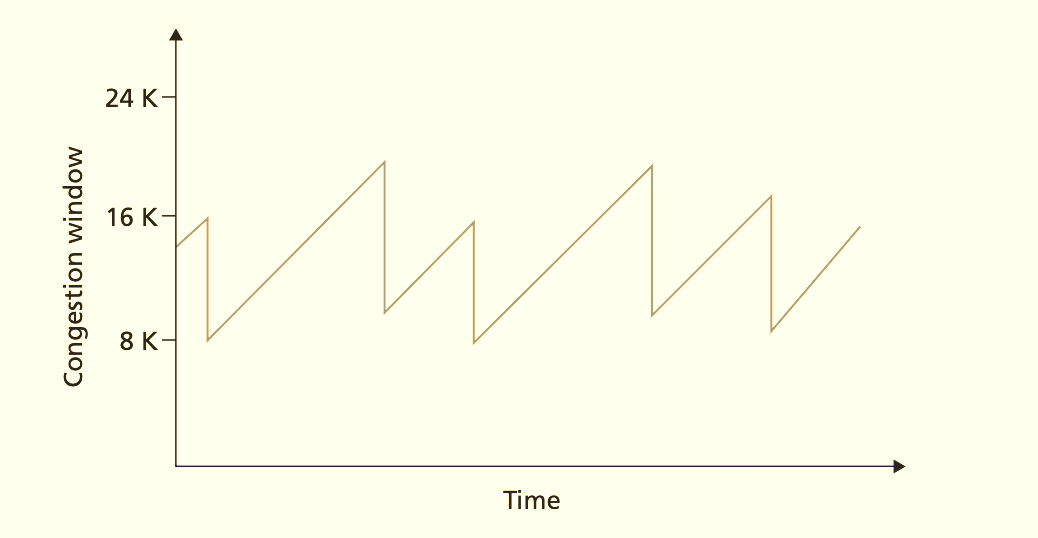
Limitations: Loss is a binary, lagging indicator. By the time a packet is dropped, the bottleneck buffer has been overfilled for an entire RTT. You have already injected cwnd worth of waste. Resetting to 1 empties the pipe completely, forcing a slow refill. The result is a sawtooth pattern: overfill, crash, underfill, overfill. Average throughput is about 75% of capacity, with periodic latency spikes equal to the buffer size.
TCP Reno:
Reno’s improvement was to recognize that not all losses are equal. Receiving three duplicate ACKs means the network is delivering most packets; only one is missing. This is mild congestion. On the other hand a timeout means catastrophic loss. The response should be proportional:
Fast Retransmit: On 3 dupACKs, retransmit the missing segment immediately.

Fast Recovery:

 ssthresh = cwnd / 2

 cwnd = ssthresh + 3 MSS // the three packets that left the network

 On each additional dupACK: cwnd += 1 MSS

 On ACK for missing segment: cwnd = ssthresh, enter Congestion Avoidance
This is a signal interpretation improvement. Three dupACKs indicate the pipe is still flowing; halve the window but don’t empty it. A timeout still triggers a full reset.
Remaining problems: You still need loss to detect congestion. The sawtooth persists, though with smaller amplitude due to fast recovery. The target is still throughput maximization, not delay minimization.
10 Gbps links
So far we have seen TCP Reno and Tahoe apply AIMD (additive increase \ multiplicative decrease) to the RTT values: The transmission rate will gradually increase until some packet loss occurs. The increase will be made by linearly increasing the congestion window, i.e. by adding a value. If congestion is inferred, the transmission ratio will be decreased, but in this case a decrease will be made by multiplying by a value. By 2004, this fundamental flaw had become acute.
Consider a 10 Gbps link with 100 ms RTT and 1460-byte segments:
With Reno, a single loss cuts cwnd from 85,616 to 42,808. Standard loss recovery takes multiple seconds. The time-to-recover compromises throughput. The sawtooth model breaks at high BDP.
CUBIC was designed for this regime.
TCP CUBIC:
TCP CUBIC takes advantage of the fact that today’s communications links tend to have increasingly higher bandwidth levels. In a network composed of wide bandwidth links, a congestion control algorithm that slowly increases the transmission rate may end up wasting the capacity of the links. The base idea was defined with BIC (Binary Increase Congestion Control). BIC’s insight was to treat bandwidth discovery as a search problem. After a loss, you know the current window is too high (congestion), and you know ssthresh is too low (safe). The available bandwidth lies somewhere between. BIC performs a binary search:
Set
W_max= pre-losscwnd(too high)Set
W_min=ssthresh(too low)Set target
W_target=(W_max + W_min) / 2Jump the window directly to
W_targetIf no loss, move
W_minup; if loss, moveW_maxdownRepeat
BIC can be too aggressive in low-RTT networks and in slower speed situations. On a 1 Mbps link with 10 ms RTT (BDP = 1.2 KB ≈ 1 segment), BIC’s binary jumps cause massive overshoot and oscillation. This led to the refinement of BIC, namely CUBIC. The intention is to have an algorithm that works with congestion windows whose incremental processes are more aggressive, but are restricted from overloading the network.
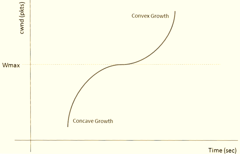
CUBIC replaces linear increase with a cubic function:W(t) = C × (t - K)³ + W_max
K = (W_max × (1 - β) / C)^(1/3)
After loss: W_max = cwnd, cwnd = β × cwnd (β ≈ 0.7), then grow along the cubic curve. Near W_max, growth is slow and stable. Far below, it’s aggressive. The use of time elapsed since the last packet loss rather than the RTT counter in cwnd adjustment makes CUBIC more sensitive to concurrent TCP sessions, particularly in short-RTT environments.
Why it became default
CUBIC replaced BIC-TCP as the present default TCP congestion control algorithm in Linux, Android, and MacOS. It is a far more efficient protocol for high speed flows and works on existing infrastructure.
High-speed performance: Recovers from loss faster than Reno.
TCP-friendly: On short RTTs, it behaves like Reno, ensuring fair convergence.
The common assumption across these flow-managed behaviours is that packet loss is largely caused by network congestion, and congestion can be avoided by reacting quickly to packet loss. But all packet losses are not entirely due to congestion. There are random wireless losses which have nothing to do with congestion.
CUBIC is still loss-based and requires overfilling buffers to find capacity, causing bufferbloat – something we’ll see again and again. It optimizes for throughput, not delay.
Kleinrock’s Power

In 1978, Leonard Kleinrock defined Power as the ratio of throughput to delay. This is the graph of power. We have packet arrival/delivery rate (G) in the network on the horizontal axis and RTT (B(G)) on the vertical axis. Note that arrival and delivery rate is not the same. But in a stable system at steady state, the arrival rate equals the delivery (departure) rate. This is a direct consequence of flow conservation (Little’s Law): On average, for every packet that arrives, one eventually leaves—otherwise, the queue would either grow infinitely (unstable) or empty out (idle server). We can safely assume both to be equal here.
Now coming back to the power diagram, for the deterministic case (when the arrival process and service process are constant), finding the optimal network operating point is easy as we increase G for as long as B(G) does not increase. This converges to β. Any further increase in sending rate will cause queueing and delay in round trip time. Buffer limit (α) is reached when the queues are filled and packet loss occurs beyond this point (recall the earlier stubborn loss-based algorithms operated at this point and completely missed the point!). The shaded region beyond a maximum sending rate (bottleneck bandwidth BtlBw) and below a minimum RTT (RTprop) is inaccessible.
For stochastic systems where one of both the arrival and service processes are random the key observation is that we cannot drive the system to utilizations that are as high as for the deterministic systems. This is because the uncertainties in the arrival times and the service times create unpredictable bunching of arrivals and variations in service times; this causes interference among the packets moving through the system and increases waiting times even when the system is not fully loaded. We call the optimal point on the dashed-power curve β`. Mathematically this point is the tangent line from the origin to the curve. More on the stochastic systems and their types in this paper. Actually the average number of packets in-flight N* = BDP.
For an M/G/1 queue (Poisson arrivals, general service distribution, one server), maximizing Power yields:
N* = 1                           // average one packet in system

ρ* = 1 / (1 + sqrt((1 + C²)/2))  // utilization < 1 to absorb variance
This state has the server always busy and the queue empty. This point also satisfies “Keep the pipe just full, and no fuller” by sending exactly as many packets as the pipe can hold without causing congestion.
In 1981, Jeffrey Jaffe proved that this optimum cannot be achieved by any decentralized algorithm. To converge to N* = BDP, each sender would need to know the sum of all other flows’ rates and the bottleneck capacity—information not locally available. Jaffe’s proof assumed:
The goal is convergence to a static operating point.
Available signals are loss and ACK timing.
Each flow acts asynchronously.
The research community pivoted correctly: from optimal to stable. Tahoe, Reno, and CUBIC are Lyapunov-stable systems converging to a fair equilibrium, not the global optimum. Jaffe’s proof held for 35 years because its assumptions were true, until measurement technology evolved.
TCP Vegas:
At its simplest, Vegas control algorithm was that an increasing RTT, or packet drop, caused Vegas to reduce its packet sending rate, while a steady RTT caused Vegas to increase its sending rate to find the new point where the RTT increased. Vegas asked why we wait for loss at all. RTT provides a continuous signal.
Define:
Expected Rate = cwnd / BaseRTT    // BaseRTT = minimum RTT ever observed

Actual Rate = cwnd / RTT          // current RTT

Diff = Expected - Actual
Diff is proportional to the number of queued packets. Vegas sets thresholds α and β (typically 1-3 MSS):
If Diff < α:      cwnd++      // under-utilizing pipe

If Diff > β:      cwnd--      // queue building, back off

Else:             cwnd unchanged  // optimal zone
This directly implements Kleinrock’s optimal point: maintain cwnd at the BDP. It is predictive—it backs off before loss occurs.
Why it failed: Fairness in a heterogeneous network.
When a Vegas flow competes with Reno flows, Reno keeps pushing until it sees loss, then backs off multiplicatively. Vegas backs off earlier, seeing RTT rise. The Reno flows eats the bandwidth Vegas yields. In game theory terms, Reno is a dominant strategy in a mixed environment. Vegas is optimal only if all flows use it. The IETF could not mandate a break with legacy behavior.
TCP BBR:
Traditional loss-based control algorithms face this impossible dilemma with buffer sizes. It fails at both extremes. The first extreme is buffer bloat. The deep buffer problem. Because memory is so cheap now. Your home router, your Wi-Fi access point, and especially those nodes in mobile networks, they often have these enormous buffers. We’re talking orders of magnitude bigger than the path actually needs to run smoothly. CUBIC sees this and starts shoving data aggressively into the pipe, keeping those huge buffers totally full. The round-trip time, which should be down in the milliseconds, suddenly blows up into seconds. That’s buffer bloat. Bandwidth is achieved but unusable because of the insane delay.
But then, almost ironically, there’s the complete opposite issue, the shallow buffers. In big data centres with modern shallow-buffer commodity switches, or perhaps more commonly for users, in wireless environments, cellular, Wi-Fi, where packet loss happens all the time just from noise or interference, not because the link is full. CUBIC sees this and immediately jumps to the wrong conclusion and cuts its sending rate down which kills the throughput.
Jaffa’s proof was critical. It showed that from any single measurement, like one RTT sample or one acknowledgment, you can’t distinguish between, say, the path getting physically longer, the available bandwidth changing, or just a queue building up. What does BBR do? How many times have we seen simple solutions win? Perhaps many.
BBR’s insight is that modern kernels can measure delivery rate directly. With microsecond-precision timestamps and kernel-level pacing, you can track:
delivery_rate = data_delivered / time_elapsed
BBR runs two independent estimators:
1. BtlBW (Bottleneck Bandwidth): Max delivery rate over a 10-RTT window. This window provides statistical averaging—noise cancels, the max captures true capacity.
2. RTprop (Round-Trip propagation time): Min RTT over the same window. Queueing noise is filtered; the min captures true propagation delay.
The BDP estimate is simply BtlBW × RTprop = BBR then paces packets to match BtlBW, using cwnd = 2 × BDP as a cap to allow burstiness. This looks like some conservation law and the first thing that comes to my mind is the equation of continuity for fluids.
The 10-RTT window is crucial. It is a distributed observer that achieves the statistical averaging Kleinrock’s stochastic theory required. Jaffe’s proof doesn’t apply because BBR isn’t solving a static optimization from local signals; it’s tracking a dynamic state using a measurement substrate that didn’t exist in 1981. BBR quietly implements Kleinrock’s 40-year-old vision.
Why BBR succeeded where Vegas failed:
Google started switching to BBR on across YouTube, Search, and Cloud, making BBR traffic a significant fraction of the internet. Globally, BBR reduced the median round-trip time by 53% on average. Think about that. Pages load faster. Searches feel instant. Fairness was redefined by market share. Vegas was technically superior to Reno but couldn’t survive in a mixed ecosystem. BBR could because Google controlled enough of the ecosystem to shift the equilibrium.
We’re ditching these indirect signs of congestion like packet loss or how full a buffer is which we’ve shown are pretty unreliable proxies. And instead we’re using this formal model based on Kleinrock’s ideas, actively measuring the path’s actual physical limits, the bottleneck bandwidth, and the base round-trip time. And maybe one of the best parts is how practical it is.
The next time you watch a 4K video with no buffering, remember: you’re seeing a control loop that measures the physics of the network 100 times per second, sending exactly the right number of packets to keep the pipe just full, but no fuller. It took four decades to make the simple idea work.
References
[1] Computer Networking - A Top-Down Approach
[2] On flow control in computer networks. L. Kleinrock